This page covers some of the basic concepts underlying FracTest, and explains some of the foundational ideas which govern the way it works.
The Mandelbrot-like fractals which FracTest renders are basically
functions on complex numbersComplex Number
Wikipedia article on complex numbers. (Wikipedia)
https://en.wikipedia.org/wiki/Complex_number.
Unfortunately, the terminology of complex numbers is somewhat
off-putting; terms like "complex", "imaginary", etc, make them sound
both difficult and artificial. In fact neither of those things is
true — complex numbers are fairly straightforward two-dimensional
numbers, and they are as much a part of the natural world as our
familiar one-dimensional numbers. Many real-world
engineering problems cannot be solved without them.
The rules of arithmetic for complex numbers are basically simple; they can be added, subtracted, multiplied, and divided, like any other numbers. There is one wrinkle, which is that the Y co-ordinate (the so-called "imaginary" part) is in units of the square root of minus one. This makes the formula for multiplication a little odd.
For our purposes, though, we can pretty much ignore this. Given the (pretty simple) rules for arithmetic with complex numbers, we can just treat them as co-ordinates. This means that they can be plotted on a graph, and displayed on a 2-dimensional computer screen, very easily. This is the basis for how fractal rendering works.
FracTest is an app which renders
fractalsFractal
Wikipedia article on fractals. (Wikipedia)
https://en.wikipedia.org/wiki/Fractal such as the
Mandelbrot setThe Mandelbrot Set
Wikipedia article on the Mandelbrot set. (Wikipedia)
https://en.wikipedia.org/wiki/Mandelbrot_set,
other similar fractals, and their related
Julia setsJulia Sets
Wikipedia article on Julia sets. (Wikipedia)
https://en.wikipedia.org/wiki/Julia_set.
The Mandelbrot set and its relatives are well covered on the Internet; however, it's worth providing a little introduction to fractal rendering here, if only to illustrate how terminology is used herein.
The Mandelbrot set is a set of complex numbers which conform to a particular criterion — specifically, that they are stable under iteration of the Mandelbrot function:
This function, as you can see, is very simple; the complexity which comes out of it is due to the nature of mathematics itself. In other words, the Mandelbrot set is something which exists in nature — it was discovered, not invented. When creating images of it, we have no control over its shape; like landscape photographers, we can choose which bits of it to take pictures of, but not what they look like.

The Mandelbrot set is drawn by mapping an area of the complex plane to the computer screen; then for each point on the screen, which represents a complex number c, we iterate the function:
The formula is iterated repeatedly on each pixel; each iteration calculates a new value for z, referred to as zn+1, based on the previous value zn, and the point c which the pixel represents. Eventually, the value of z will do one of two things:
In the first case, the point c is inside the Mandelbrot set, and is coloured black. In the second case, the point is outside the Mandelbrot set, and we colour it according to your selected representation function, as described below. Typically this will involve the number of iterations it took to escape past a distance of 2.0 (or whatever bailout value you have configured).
This simple formula is responsible for all of the infinite complexity, and infinite beauty, in the Mandelbrot set.

FracTest provides controls to pick which area in the complex plane is mapped to the screen (specified as its centre and size). In FracTest, the size of an area of the fractal is defined by what we call the "radius", which is actually half the height.
Starting from the overall view of the Mandelbrot set, you can explore it by picking an interesting point to zoom in on, usually by using a selection. Then, repeat the process. As you zoom farther in, the number of digits in the co-ordinates increases, and FracTest will switch to more complex maths modes to cope — you will notice it slowing down. Very zoomed-in views are referred to as "deep", and going deep needs a lot of maths to compute the image.
The way a Mandelbrot set point is converted to a visible colour is called the representation function. There are many possible representation functions, but FracTest only supports a few; these can be used in any combination, and the colours generated by them will be averaged. You can select the function or functions to use in the user interface.
The supported representation functions are:
This is the most widely-used and simple function; although it's easy to compute, it gives a useful idea of how "close" a given point is to the Mandelbrot Set, and hence gives a good idea of the true shape of the set.
This function illustrates how regions of the Mandelbrot set are influenced by nearby satellites. It does not show the shape of the set itself, but it is of interest when exploring the relationships between structures within the set.
Note that when using this function, the bailout value should be set to a high value to obtain a detailed plot.
Each of the infinitely many points in and around the Mandelbrot set has
a corresponding Julia setJulia Sets
Wikipedia article on Julia sets. (Wikipedia)
https://en.wikipedia.org/wiki/Julia_set, which itself
is an infinitely complex fractal. FracTest allows these Julia sets to
be computed.
For a specific point r in the complex plane — and particularly where r is an interesting point in the Mandelbrot set — a Julia set is drawn by similarly mapping an area of the complex plane to the computer screen; then for each point on the screen, representing a complex number c, we iterate the function:
The difference is that z starts at c, the screen
point we're displaying; but the additive term is r, the Julia
set reference point, which is the same for all points on the screen.
The main effort by far in generating a fractal view is mathematical calculations, and many of them. A typical high-resolution view can easily involve many trillions of individual additions, subtractions, and multiplications, which might take hours or days. Making these as fast as possible is obviously a key goal.
However, the more deeply you zoom into the fractal, the more digits are required to correctly calculate the co-ordinates of the individual pixels so that they can be computed correctly. As you zoom deeper, you need more digits.
The fastest way to do maths in a computer is by using its built-in arithmetic hardware. This is very fast, since it ultimately comes down to networks of transistors wired to produce the result electrically; however, the number of digits in the result is strictly limited. Specifically, the data type is called double, and it has a precision of 53 bits, which is around 15-16 decimal digits. At a zoom level over 1013 — in other words, when zoomed in 10 thousand billion times — the processor's arithmetic hardware reaches the limit of its resolution. Any attempt to zoom farther will produce pixellated images.
This might seem like a pretty remote limit, but in fact when exploring Mandelbrot in depth, it's pretty easy to get that far in and hit the wall. Since FracTest is designed for in-depth exploration, it's important to have a means to perform arithmetic with more precision. The answer is software arithmetic, where software is used to perform calculations instead of the machine's hardware. This allows any amount of precision you like (memory is really not an issue), but the expense is speed — a general-purpose software maths package can easily be 300 times slower, or more, than hardware. And it only gets slower as you zoom in, and the number of digits you need goes up.
FracTest has two software maths packages, each offering the best available performance at particular resolutions. So in all, there are 3 modes for arithmetic:
HW): using the machine's native double
arithmetic hardware, this is by far
the fastest mode, but limited to zooms of around 1013.DD): a technique developed by David Bailey and Yozo Hida
where two hardware numbers are combined in software to make a larger
value, with around 106 bits, or 30 decimal places, of precision.
This is about 20 times slower than hardware, but allows zooms up
to around 1030.FX-nn): a
fixed-precision library developed specifically for FracTest, based on
Knuth's algorithmsThe Art of Computer ProgrammingDD at the same
resolution, but allows unlimited precision. It is also very fast compared to
other unlimited-precision libraries. The suffix nn is the
number of 32-bit words used to store the fractional part in the current
view, so the precision is 32 times nn in bits, or about
10 times nn in decimal digits.Fixed mode is a little complicated. An individual Fixed value has a fixed
precision, i.e. a specific number of fraction bits; although Fixed
actually measures precision in 32-bit words. A Fixed value can be
created at any size, but then stays at that size as we do arithmetic on
it. As you zoom deeper, FracTest will automatically create Fixed
values with larger precisions. So, Fixed is more like a set of
modes rather than a specific mode — FX-12 offers more
precision than FX-10, etc. If you leave the Math Mode at
AUTO, this pretty much takes care of itself; but if you set
the mode manually, remember that you will need to specify the appropriate
precision as you zoom deeper. The
resolution indicator in the
main window will show you how much precision you have left at the
current mode.
A practical consequence of all this is that if you leave the Math Mode
at AUTO (which is generally a good idea), then as you zoom in you
will hit a point where the render suddenly becomes much slower, as FracTest
switches to software arithmetic. It will then keep on getting slower as you zoom
deeper.
The example at right is a fractal view
at a zoom level of 106,566 — a 1 with 6,566 zeros after it;
this was computed using FX-682 mode, which provides 21,818 bits of
precision. Even at the very low resolution of 480x270 pixels, this took
over 3.3 days to render on a cluster with 34 processors.
It's a widely-held belief that computers keep getting faster; and like many widely-held beliefs, it's wrong. Pentium 4 (Prescott) CPUs reached 3.8 GHz in 2004; modern (2018, 7th-gen Core i7) CPUs are at around the same speed. Of course, there have been advances in computer performance in the intervening 14 years, but these have been realised through more efficient architectures, and also through parallel processing — packing multiple CPUs ("cores") into a single chip so that it can do more.
The problem with the multi-core approach is that any plainly-written software can only run on one CPU at a time. In an 8-core machine, with one "regular" app running flat out, 7 CPUs will be idle and therefore not adding any performance. To get the benefit of multiple cores, you either have to have multiple programs running at once — and actually running, not just open on the screen — or you need software which is written to break a task down into multiple parts and run them in parallel. This is referred to as multi-threading. It's quite hard to do this, and so most general apps are not written to be multi-threaded; but fortunately fractal rendering is just about the easiest thing to make multi-threaded.
FracTest implements multi-threading by dividing a view into tiles. These are small rectangular areas of the view, each of which is an independent unit of work, which can be computed on its own; so with multiple processors, we can have multiple tiles — one per processor — being computed at one time. This allows all the available processors to be utilised fully, giving us the fastest possible computation.
The size, and hence number, of tiles depends on the view parameters. Generally we want each tile to be big enough to allow for progressive rendering, but not so big that some processors can finish leaving others with substantial work to do. This latter point is particularly relevant when using a compute cluster which may have many processors.
FracTest splits the image into tiles based on the current progressive rendering mode. So, if you are computing a low-resolution image, you should keep progressive rendering to a low number of passes. This will allow many tiles to be created, which will help to split the work across all available processors.
The information panel in the main window shows the number of tiles the view has been divided into, and how many pixels there are in each tile. You can see these tiles during a computation, when the active tiles are drawn as boxes on the main fractal view.
The same technique which allows FracTest to utilise all the cores in a single computer also works with multiple computers on a network. FracTest can send tiles over the network to remote servers, have them computed there, and then send the results back to be integrated into the fractal view. This allows for large views to be computed in a feasible amount of time, by throwing large numbers of processors at the problem.
In fact, FracTest always uses compute servers to do the work — if you don't set up any remote servers, it will create an internal server to do the work on the local machine. This is invisible to the user, so it looks as if FracTest is a simple monolithic application.
One issue which complicates things a little is the relatively recent
development of hyper-threadingHyper-threading
An article on hyper-threading, used in modern computers to increase performance with minimal added cost. (Wikipedia)
https://en.wikipedia.org/wiki/Hyper-threading.
Basically, this involves each CPU
masquerading as 2 CPUs, which then allows them to utilise time which
would otherwise be wasted, for example waiting for data to arrive from
main memory. So with hyper-threading, your computer will report
having twice as many CPUs as it actually has; and you will gain a bit
more than the performance of the true number of CPUs, but for a lot
less cost than doubling them.
The actual benefit you get from hyper-threading depends very strongly on the app. However, on my system, I see about a 50% improvement from it in FracTest (in other words, I have 4 CPUs, reporting themselves as 8 CPUs, and giving me roughly the performance of 6 CPUs).
We use the term "logical CPUs" to denote the number of processors reported by hyper-threading; so on most modern systems, the number of logical CPUs will be twice the number of actual physical processors. To get the benefit of hyper-threading, the number of threads we want to create is based on the number of logical (not physical) CPUs; so FracTest will always report this number.
There are several kinds of information you might want to save while exploring a fractal:
Fortunately, there is a way we can save all of this information in a single file. Modern media files are not just simply the media data (such as a picture) shoved into a file; they are multi-part containers, which provide for many different kinds of information to be saved along with the media. This extra information is generically called meta-data, and it can be used for just about anything.
FracTest uses the meta-data of a
PNG (Portable Network Graphics)Portable Network Graphics
Article on the PNG lossless image file format. (Wikipedia)
https://en.wikipedia.org/wiki/Portable_Network_Graphics file to
save all of the information relevant to a fractal
view in one file. The image part of the PNG file is the computed image,
and the other information is saved as meta-data. This makes life
very simple, as any saved fractal image contains not just the image,
but all the parameters used to render it.
When you load a PNG file in FracTest, the fractal parameters are loaded, and the fractal image is re-rendered. This is extremely useful when you see an image you want to make adjustments to — just load the image, and you can adjust the colours, or change the resolution, or just continue exploring the fractal from where you left off. Better yet, if the image contains a valid computation state, the image will be re-computed from where the computation left off, and if the computation had finished, the finished image will be displayed immediately.
You can also load just the colour palette from a PNG file. Hence, PNG files can be used to store useful palettes.
Altogether, then, the PNG file as created by FracTest serves multiple purposes:
The FracTest files page describes all of this in more detail.
FracTest supports simple sub-pixel anti-aliasing. When turned on, each pixel will be divided into a specified number of sub-pixels; these will be calculated, converted to colours, and then averaged to produce the final pixel colour. The effect is as if the image had been generated at a higher resolution and then scaled down, but without the memory requirement that would be needed for the larger image.
FracTest names its anti-aliasing modes according to how many sub-pixels are used per pixel; hence "4" means that each pixel is broken into a grid of 2×2 sub-pixels.
Each anti-aliasing mode therefore indicates the performance penalty: with AA at "9", the fractal will take 9 times longer to compute than with AA off. The result will, however, look much better. "16" is very high; the difference to "9" is subtle, but visible to close inspection.
Progressive rendering means that a fractal view is computed very roughly at first, by only computing a sampling of the pixels; then filled in with more detail as time goes on. FracTest provides a user-selectable choice of progressive rendering modes from none (pixels are done top-to-bottom) to 6-pass.
The benefit of progressive mode is that you can very quickly see how a fractal view will look, at least in broad terms. Even before 1% of the calculation is done, you can see what shape it is, how it is framed, and roughly how the colours look. This is invaluable when exploring, as it lets you very quickly make adjustments to get to the view you want.
Still, progressive mode is very useful. A full understanding of how it actually works might help you to get the best from it.
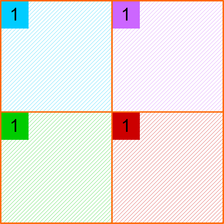
To illustrate by example, three-pass progressive mode would work as follows. In pass 1, the image is divided into 4×4 pixel boxes. The upper left pixel in each box — that is, every 4th pixel horizontally and vertically — is calculated, and the entire box is coloured according to the calculated value. This is illustrated at right.
Only 1 in 16 pixels is actually calculated, making this very fast. Of course the visual result is very coarse.
Note that if anti-aliasing is turned on, each pixel is calculated with full anti-aliasing, so that the computed pixels (shown numbered in the diagram) are set to their final values.

The image at the right shows the state of affairs after pass 2. Only the pixels numbered 2 are calculated in this pass; each 2×2 sub-block is coloured according to the calculated pixels. The top-left sub-block in each original 4×4 block retains its colour from pass 1.

The image at right shows the final state. Again, only the pixels numbered 3 are calculated in this pass.
The end result of all this:
no pixel is calculated twice; we just do them in a non-linear order.
each pass does 3 times as much work as the previous pass. Things therefore slow down very quickly. One third of the final pass will be done before you are at 50% of a computation.
progressive mode requires blocks of pixels to work in; for example 4×4 pixels for three passes. The size doubles for each additional pass. Since the progressive organisation happens within tiles, it can't work if the tile isn't big enough. This is why we limit progressive to 6 passes, though that is easily enough for most purposes.
there is slightly higher overhead in managing the calculations and re-calculations of tiles. If a tile is calculated very fast, and if the progressive mode means that only 2 pixels are calculated in a tile on pass 1 (which can happen), then the ratio of overhead to calculation becomes high on the first passes. Therefore using many progressive passes on a fast image can slow things down a little; but if the image is fast anyway, it's generally not a big deal.
One additional benefit of progressive mode is that after pass 1, we have a rough idea of how long each tile takes to render, based on the pixels calculated so far. Since we have only computed a sampling of the pixels this will be approximate, but it can be enough to tell us that a tile in the black centre of an image may take much longer to compute than a tile near the edge.
This information is used after pass 1 to make a more accurate guess at the time remaining in a computation, by taking into account the actual work done for each tile — this is shown in the bottom status bar. (In pass 1, the percentage complete is based on a simple pixel count.) It is also used to order the tiles so that the slowest tiles are computed first on subsequent passes. This is done primarily for efficiency — by getting the slow tiles out of the way first, we can use the more fine-grained work units (the faster tiles) to keep all the available processors running to the end.